
What is the Proportional Odds Assumption?
To assume proportional odds is to declare the effects of any explanatory variables to be the same across different thresholds. These thresholds are the splits between each pair of categories of the ordinal outcome variable. The coefficients for each predictor category must be consistent, or have parallel slopes, across all levels of the response. In ordinal regression, there will be separate intercept terms at each threshold, but a single odds ratio (OR) for the effect of each explanatory variable.
When should the Proportional Odds Model be used?
We can use it when there are two or more outcome categories that have a specific order. Examples include quiz answers ranging from Strongly Disagree to Strongly Agree, rating something from 1 to 10, and disease severity of ‘mild’, ‘moderate’, or ‘severe’.
What is the score test for the Proportional Odds Assumption?
The score test is based upon the assumption that the null hypothesis is true – the explanatory variables effects having a constant effect across categories. The score statistic is defined as where both the score function and Fisher information matrix are evaluated at the MLE under the null hypothesis, θ. Under the null hypothesis, the score statistic also follow the X2 distribution with (J-2)s degrees of freedom.
Below, we present an example from the University of Virginia [1], which uses the programming language R.
Fitting and Interpreting a Proportional Odds Model
The following table is a cross tabulation of data taken from the 1991 General Social Survey that relates political party affiliation to political ideology.
| Very Liberal | Slightly Liberal | Moderate | Slightly Conservative | Very Conservative | |
| Republican | 30 | 46 | 148 | 84 | 99 |
| Democratic | 80 | 81 | 171 | 41 | 55 |
What if we wanted to model the probability of answering a particular political ideology given party affiliation? Since the political ideology categories have an ordering, we would want to use ordinal logistic regression. We will run the model in R first and then explain afterwards.
# Table 8.6, Agresti 1996
party <- factor(rep(c("Rep","Dem"), c(407, 428)),
levels=c("Rep","Dem"))
rpi <- c(30, 46, 148, 84, 99) # cell counts
dpi <- c(80, 81, 171, 41, 55) # cell counts
ideology <- c("Very Liberal","Slightly Liberal","Moderate","Slightly Conservative","Very Conservative")
pol.ideology <- factor(c(rep(ideology, rpi),
rep(ideology, dpi)), levels = ideology)
dat <- data.frame(party,pol.ideology)
# fit proportional odds model
library(MASS)
pom <- polr(pol.ideology ~ party, data=dat)
Above, we create a data frame with one row for each respondent. The first column we create is party, with 407 entries for Republican and 428 for Democratic. The next column we create is pol.ideology. We use the cell counts (stored as rpi and dpi, respectively) with the rep() function to repeat each ideology a given number of times. For example, rep(ideology, rpi) repeats "Very Liberal" 30 times, "Slightly Liberal" 46 times, and so on. Finally we create a data frame called dat. We fit the model using the polr() function from the MASS package. "polr" stands for proportional odds logistic regression. The MASS package comes with R. Let's look at the model summary:
summary(pom)
Call:
polr(formula = pol.ideology ~ party, data = dat)
Coefficients:
Value Std. Error t value
partyDem -0.9745 0.1292 -7.545
Intercepts:
Value Std. Error t value
Very Liberal|Slightly Liberal -2.4690 0.1318 -18.7363
Slightly Liberal|Moderate -1.4745 0.1090 -13.5314
Moderate|Slightly Conservative 0.2371 0.0942 2.5165
Slightly Conservative|Very Conservative 1.0695 0.1039 10.2923
Residual Deviance: 2474.985
AIC: 2484.985
We have one coefficient and four intercepts. Let's move ahead with using our model to make predictions. Below we use our model to generate probabilities for answering a particular ideology given party affiliation:
predict(pom,newdata = data.frame(party="Dem"),type="p")
Very Liberal Slightly Liberal Moderate Slightly Conservative Very Conservative
0.1832505 0.1942837 0.3930552 0.1147559 0.1146547
predict(pom,newdata = data.frame(party="Rep"),type="p")
Very Liberal Slightly Liberal Moderate Slightly Conservative Very Conservative
0.07806044 0.10819225 0.37275214 0.18550357 0.25549160
The newdata argument requires data be in a data frame, hence the data.frame() function. The type="p" argument says we want probabilities. To explain where these results came from, we need to look at the proportional odds model:
![]()
On the right side of the equal sign we see a simple linear model with one slope, β, and an intercept that changes depending on j, αj. Here the j is the level of an ordered category with J levels. In our case, j = 1 would be "Very Liberal." So we see we have a different intercept depending on the level of interest. Why does j only extend to J - 1? Because in this model we're modelling the probability of being in one category (or lower) versus being in categories above it. In our example, P(Y≤2) means the probability of being "Very Liberal" or "Slightly Liberal" versus being "Moderate" or above. Thus we're using the levels as boundaries. In this model the highest level returns a probability of 1 (i.e., P(Y≤J)=1), so we don't model it. Now what about the logit? That means log odds. It's not the probability we model with a simple linear model, but rather the log odds of the probability:
.png?width=104&height=55&name=Proportional%20Odds%20Assumptions%20Equation%20(1).png)
If probability is 0.75, the of 0.75 is log(0.75/(1-0.75))=1.09. The summary output of our model is stated in terms of this model. Since we have 5 levels, we get 5 - 1 = 4 intercepts. We have one predictor, so we have one slope coefficient. Plugging in values returns estimated log odds. Let's try this. What are the log odds a Democrat identifies as "Slightly Liberal" or lower? Plug in the appropriate values from the model output given above:
![]()
Let's convert to probability. This means taking the inverse logit. The formula for this is:
.png?width=283&height=66&name=Proportional%20Odds%20Assumptions%20Equation%20(3).png)
Applying to -0.5 we get:
.png?width=330&height=74&name=Proportional%20Odds%20Assumptions%20Equation%20(4).png)
This is cumulative probability. The probability of identifying as "Very Liberal" or "Slightly Liberal" when you're a Democrat is about 0.378. This is why the labels for the intercepts in the summary output have a bar ("|") between the category labels: They identify the boundaries. So how did R calculate the probabilities for being in a particular category? In other words, how do we calculate P(Y=j)? We do some subtraction:
![]()
For example, the probability of a Democrat identifying as "Slightly Liberal" is:
![]()
The baseline level in this model is Republican, so we set x = 0 when doing their calculations. The probability of a Republican identifying as "Slightly Liberal" or lower is simply:
.png?width=502&height=76&name=Proportional%20Odds%20Assumptions%20Equation%20(7).png)
We can speed up these calculations by using elements of the pom object. The slope coefficient is stored in pom$coefficient and the intercepts are stored in pom$zeta. (The developers of the polr() function like using zeta to represent the intercepts instead of alpha). Here's how to quickly calculate the cumulative ideology probabilities for both Democrats and Republicans:
# Democrat cumulative probabilities
exp(pom$zeta - pom$coefficients)/(1 + exp(pom$zeta - pom$coefficients))
Very Liberal|Slightly Liberal Slightly Liberal|Moderate
0.1832505 0.3775341
Moderate|Slightly Conservative Slightly Conservative|Very Conservative
0.7705894 0.8853453
# Republican cumulative probabilities
exp(pom$zeta)/(1 + exp(pom$zeta))
Very Liberal|Slightly Liberal Slightly Liberal|Moderate
0.07806044 0.18625269
Moderate|Slightly Conservative Slightly Conservative|Very Conservative
0.55900483 0.74450840
That hopefully explains the four intercepts and one slope coefficient. But why the name "proportional odds"? "Proportional" means that two ratios are equal. Recall that odds is the ratio of the probability of success to the probability of failure. In this case, "success" and "failure" correspond to P(Y≤j) and P(Y>j), respectively. The ratio of those two probabilities gives us odds. We can quickly calculate the odds for all J-1 levels for both parties:
# Democrat cumulative probabilities
dcp <- exp(pom$zeta - pom$coefficients)/(1 + exp(pom$zeta - pom$coefficients))
# Republican cumulative probabilities
rcp <- exp(pom$zeta)/(1 + exp(pom$zeta))
# Democrat odds
(dcp/(1-dcp))
Very Liberal|Slightly Liberal Slightly Liberal|Moderate
0.2243656 0.6065138
Moderate|Slightly Conservative Slightly Conservative|Very Conservative
3.3589956 7.7218378
# Republican odds
(rcp/(1-rcp))
Very Liberal|Slightly Liberal Slightly Liberal|Moderate
0.0846698 0.2288827
Moderate|Slightly Conservative Slightly Conservative|Very Conservative
1.2675986 2.9140230
Now, let's take the ratio of the Democratic ideology odds to the Republican ideology odds:
(dcp/(1-dcp))/(rcp/(1-rcp))
Very Liberal|Slightly Liberal Slightly Liberal|Moderate
2.649889 2.649889
Moderate|Slightly Conservative Slightly Conservative|Very Conservative
2.649889 2.649889
Look, they're all the same. The odds ratios are equal, which means they're proportional. And now we see why we call this a proportional odds model. For any level of ideology, the estimated odds that a Democrat's response is in the liberal direction (to the left) rather than the conservative direction is about 2.6 times the odds for Republicans.
log((dcp/(1-dcp))/(rcp/(1-rcp)))
Very Liberal|Slightly Liberal Slightly Liberal|Moderate
0.9745178 0.9745178
Moderate|Slightly Conservative Slightly Conservative|Very Conservative
0.9745178 0.9745178
Does that number look familiar? It's the slope coefficient in the model summary, without the minus sign. Some statistical programs, like R, tack on a minus sign so higher levels of predictors correspond to the response falling in the higher end of the ordinal scale. If we exponentiate the slope coefficient as estimated by R, we get exp(-0.9745) = 0.38. This means the estimated odds that a Democrat's response in the conservative direction (to the right) is about 0.38 times the odds for Republicans. That is, they're less likely to have an ideology at the conservative end of the scale.
Testing the Assumption of Proportional Odds
One way of testing this assumption is the Brant-Wald test, which we will demonstrate using an example from People Analytics [2] in R. A proportional odds regression model effectively acts as a series of stratified binomial models under the assumption that the ‘slope’ of the logistic function of each stratified model is the same. This can be verified by running stratified binomial models on our data and checking for similar coefficients on our input variables. Here we have an example of football data on players being disciplined by the referee for unfair or dangerous play. We are provided with data on over 2000 different players in different games, and the data contains these fields:
- discipline: A record of the maximum discipline taken by the referee against the player in the game. ‘None’ means no discipline was taken, ‘Yellow’ means the player was issued a yellow card (warned), ‘Red’ means the player was issued a red card and ordered off the field of play.
- n_yellow_25 is the total number of yellow cards issued to the player in the previous 25 games they played prior to this game.
- n_red_25 is the total number of red cards issued to the player in the previous 25 games they played prior to this game.
- position is the playing position of the player in the game: ‘D’ is defence (including goalkeeper), ‘M’ is midfield and ‘S’ is striker/attacker.
- result is the result of the game for the team of the player—‘W’ is win, ‘L’ is lose, ‘D’ is a draw/tie.
Firstly, our outcome of interest is discipline and this needs to be an ordered factor, which we can choose to increase with the seriousness of the disciplinary action.
# convert discipline to ordered factor
soccer$discipline <- ordered(soccer$discipline,
levels = c("None", "Yellow", "Red"))
We then run our model:
# run proportional odds model
library(MASS)
model <- polr(
formula = discipline ~ n_yellow_25 + n_red_25 + position +
result,
data = soccer
)
# get summary
summary(model)
## Call:
## polr(formula = discipline ~ n_yellow_25 + n_red_25 + position +
## result, data = soccer)
##
## Coefficients:
## Value Std. Error t value
## n_yellow_25 0.32236 0.03308 9.7456
## n_red_25 0.38324 0.04051 9.4616
## positionM 0.19685 0.11649 1.6899
## positionS -0.68534 0.15011 -4.5655
## resultL 0.48303 0.11195 4.3147
## resultW -0.73947 0.12129 -6.0966
##
## Intercepts:
## Value Std. Error t value
## None|Yellow 2.5085 0.1918 13.0770
## Yellow|Red 3.9257 0.2057 19.0834
##
## Residual Deviance: 3444.534
## AIC: 3464.534
We can see that the summary returns a single set of coefficients on our input variables as we expect, with standard errors and t-statistics. We also see that there are separate intercepts for the various levels of our outcomes, as we also expect. In interpreting our model, we generally don’t have a great deal of interest in the intercepts, but we will focus on the coefficients. We can interpret them as follows, in each case assuming that other coefficients are held still:
- Each additional yellow card received in the prior 25 games is associated with an approximately 38% higher odds of greater disciplinary action by the referee.
- Each additional red card received in the prior 25 games is associated with an approximately 47% higher odds of greater disciplinary action by the referee.
- Strikers have approximately 50% lower odds of greater disciplinary action from referees compared to Defenders.
- A player on a team that lost the game has approximately 62% higher odds of greater disciplinary action versus a player on a team that drew the game.
- A player on a team that won the game has approximately 52% lower odds of greater disciplinary action versus a player on a team that drew the game.
As we learned, proportional odds regression models effectively act as a series of stratified binomial models under the assumption that the ‘slope’ of the logistic function of each stratified model is the same. We can verify this by running stratified binomial models on our data and checking for similar coefficients on our input variables. Let’s create two columns with binary values to correspond to the two higher levels of our ordinal variable.
# create binary variable for "Yellow" or "Red" versus "None"
soccer$yellow_plus <- ifelse(soccer$discipline == "None", 0, 1)
# create binary variable for "Red" versus "Yellow" or "None"
soccer$red <- ifelse(soccer$discipline == "Red", 1, 0)
Now let’s create two binomial logistic regression models for the two higher levels of our outcome variable.
# model for at least a yellow card
yellowplus_model <- glm(
yellow_plus ~ n_yellow_25 + n_red_25 + position +
result,
data = soccer,
family = "binomial"
)
# model for a red card
red_model <- glm(
red ~ n_yellow_25 + n_red_25 + position +
result,
data = soccer,
family = "binomial"
)
We can now display the coefficients of both models and examine the difference between them.
(coefficient_comparison <- data.frame(
yellowplus = summary(yellowplus_model)$coefficients[ , "Estimate"],
red = summary(red_model)$coefficients[ ,"Estimate"],
diff = summary(red_model)$coefficients[ ,"Estimate"] -
summary(yellowplus_model)$coefficients[ , "Estimate"]
))
## yellowplus red diff
## (Intercept) -2.63646519 -3.89865929 -1.26219410
## n_yellow_25 0.34585921 0.32468746 -0.02117176
## n_red_25 0.41454059 0.34213238 -0.07240822
## positionM 0.26108978 0.06387813 -0.19721165
## positionS -0.72118538 -0.44228286 0.27890252
## resultL 0.46162324 0.64295195 0.18132871
## resultW -0.77821530 -0.58536482 0.19285048
Ignoring the intercept, which is not of concern here, the differences appear relatively small. Large differences in coefficients would indicate that the proportional odds assumption is likely violated and alternative approaches to the problem should be considered.
In this, some judgment is required to decide whether the coefficients of the stratified binomial models are ‘different enough’ to decide on violation of the proportional odds assumption. For those requiring more formal support, an option is the Brant-Wald test. Under this test, a generalized ordinal logistic regression model is approximated and compared to the calculated proportional odds model. A generalized ordinal logistic regression model is simply a relaxing of the proportional odds model to allow for different coefficients at each level of the ordinal outcome variable.
The Wald test is conducted on the comparison of the proportional odds and generalized models. A Wald test is a hypothesis test of the significance of the difference in model coefficients, producing a chi-square statistic. A low p-value in a Brant-Wald test is an indicator that the coefficient does not satisfy the proportional odds assumption. The brant package in R provides an implementation of the Brant-Wald test, and in this case supports our judgment that the proportional odds assumption holds.
library(brant)
brant::brant(model)
## --------------------------------------------
## Test for X2 df probability
## --------------------------------------------
## Omnibus 14.16 8 0.08
## n_yellow_25 0.24 1 0.62
## n_red_25 1.83 1 0.18
## positionM 1.7 1 0.19
## positionS 2.33 1 0.13
## resultL 1.53 1 0.22
## resultW 1.3 1 0.25
## --------------------------------------------
##
## H0: Parallel Regression Assumption holds
A p-value of less than 0.05 on this test—particularly on the Omnibus plus at least one of the variables—should be interpreted as a failure of the proportional odds assumption.
What is a violation of the Proportional Odds Assumption?
The proportional odds assumption may be violated if the p values are below the designated threshold, for example 0.05. If we use stratified binomial models and they show that the effects of the categorical variables differ between ordinal thresholds, this also suggests that the proportional odds violation doesn’t hold, and that we should consider other models.
There are many other tests such as likelihood testing, the score test, the Wolfe-Gould test, the Lipsitz test, and the Pulkstenis-Robinson test, among others. The score test is widely used in practice as it is the only test directly available in SAS; however, its controlling of type I error is not very good. For small samples, generally, it may reject much more often than the nominal type I error level indicates. The same is true for the Wald and LR tests. On the other hand, the Brant and Wolfe-Gould tests generally control the type I error quite well. Thus, the Brant and Wolfe Gould tests are usually recommended when the sample size is small [3].
When the proportional odds assumption is rejected, we may assess the cause of the violation. For a very large sample, we may obtain significant results even when the proportional odds assumption is slightly violated. In such a case, it may still be practical to apply the proportional odds models. Otherwise, we may need to revise the model.
Partial Proportional Odds Models
What if the assumption of proportional odds only works for some variables? We present an example of a large randomised study of 19,285 individuals [4] using SAS 9.3 to highlight the advantages and pitfalls of ordinal logistic regression where there may be doubt in the strength of the proportional odds assumption.
Ordinal Scale
Physical ability and dependency on care is assessed at six months following a stroke event, typically using an ordinal scale of ordered categories ranging from complete or partial recovery to dependency and death. From Figure 1, we can see that a slight shift towards the lower scores and away from higher scores in individuals treated with aspirin in the IST.
Figure 1: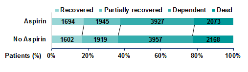
Using a binary logistic model, we can see from Figure 2 that a small effect of aspirin is observed, however, the effect is not significant no matter the chosen partition of the outcome scale.
Figure 2:
Performing ordinal logistic regression, we can produce a common odds ratio, which has a narrower confidence interval, suggesting this method has greater power to detect a significant effect, although this method is performed under the assumption of proportional odds.
The proportional odds assumption means that for each term included in the model, the 'slope' estimate between each pair of outcomes across two response levels are assumed to be the same regardless of which partition we consider. A test of the proportional odds assumption for the aspirin term indicates that this assumption is upheld (p=0.898).
A potential pitfall is that the proportional odds assumption continues to apply when additional parameters are included in the model. Guidelines from the Committee for Medicinal Products for Human Use (CHMP) published in 2013 [5] recommend using adjusted analyses which include baseline covariates significantly related to the outcome. Related covariates typically improve the fit of the model, however, in this case adding age, sex and consciousness on admission to hospital to the model causes the proportional odds assumption to be rejected (p<0.001). This means the assumption of proportional odds is not upheld for all covariates now included in the model.
Benefits of Ordinal Logistic Regression – Exploring Proportionality of Data
In SAS version 9.3 or higher, options now exist to better explore the proportionality of your data using PROC logistic. Specifying ‘unequalslopes’ removes the assumption that coefficients are equal between categories and instead produces an estimate for each model term at each partition of the scale. The results can be viewed in Table 1.
PROC logistic data = asp_data order=internal outest=varlabels;
class asp conscious sex / param = ref;
/* Specify unequal slopes to obtain estimates for each model term at each partition of the outcome scale */
model score = asp age conscious sex / unequalslopes;
RUN;
Table 1:
|
Analysis of Maximum Likelihood Estimates |
||||
|
Parameter |
Estimate |
95% Wald CL |
Pr > ChiSq |
|
|
Aspirin |
1 |
1.075 |
0.996, 1.161 |
0.0650 |
|
2 |
1.068 |
1.003, 1.137 |
0.0399 |
|
|
3 |
1.073 |
0.996, 1.155 |
0.0619 |
|
|
Age (per 10 yrs older) |
1 |
0.737 |
0.714, 0.762 |
<.0001 |
|
2 |
0.597 |
0.580, 0.615 |
<.0001 |
|
|
3 |
0.533 |
0.513, 0.555 |
<.0001 |
|
|
Conscious |
1 |
4.878 |
4.225, 5.632 |
<.0001 |
|
2 |
5.982 |
5.411, 6.613 |
<.0001 |
|
|
3 |
5.010 |
4.637, 5.412 |
<.0001 |
|
|
Males versus Females |
1 |
1.260 |
1.164, 1.365 |
<.0001 |
|
2 |
1.378 |
1.292, 1.470 |
<.0001 |
|
|
3 |
0.899 |
0.833, 0.970 |
0.0063 |
|
These test statements can be included under the model statement to test the proportional odds assumption for each covariate of the model. The results of these tests can be seen in Table 2.
/* Test partition estimates */
Aspirin: test asp1_1 = asp1_2 = asp1_3;
Age: test age_1 = age_2 = age_3;
Conscious: test conscious1_1 = conscious1_2 =conscious1_3;
Sex: test sex1_1 = sex1_2 = sex1_3;
RUN;
Table 2:
|
Linear Hypotheses Testing Results |
|||
|
Label |
Wald |
DF |
Pr > ChiSq |
|
Aspirin |
0.0484 |
2 |
0.9761 |
|
Age (per 10 years older) |
237.8197 |
2 |
<.0001 |
| Conscious |
21.5721 |
2 |
<.0001 |
|
Males vs. Females |
101.7181 |
2 |
<.0001 |
Table 1 shows us that the effect of aspirin is roughly constant over the scale and the hypothesis test in Table 2 indicates that the assumption of proportional odds holds for this parameter. We can see that you are less likely to improve with each 10 years of age and that improvement becomes even less likely with each increase in score on the outcome scale and thus the proportional odds assumption does not hold for this parameter. Similarly, the effect of consciousness is not constant across the scale, shown by rejection of the hypothesis test, however, being conscious upon admission to hospital confers significant benefit to your recovery after six months. Males were observed to have lower scores than females in the lower score categories but being male was observed to confer greater risk of death overall and consequently does not uphold the assumption of proportional odds.
Presenting a Partially Proportional Model
The proportionality restriction can be relaxed within the PROC logistic procedure for only those covariates not meeting the assumption. In this case, the model statement can be modified to specify unequal slopes for age, consciousness and sex using the following syntax. Figure 3 shows graphically the model estimates obtained from a partially proportional model, while a likelihood ratio test revealed that this model fitted significantly better than a fully non-proportional model. The advantage of the partial proportional model is that a common estimate for aspirin can be obtained, while non-proportional parameters are not constrained.
model score = asp age conscious sex
/ unequalslopes=(age conscious sex);
Figure 3:
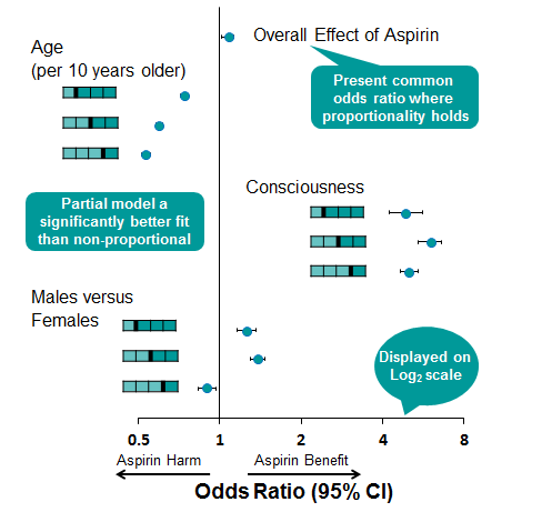
By using PROC logistic to perform an ordinal logistic regression model, we have produced a more efficient estimate of the effect of aspirin and have several tools to explore the proportionality of data and adjust the proportionality restriction for only those covariates where the assumption is not upheld. The pitfalls in using this type of model are that potential treatment harm can be masked by a single common odds estimate where the data have not been fully explored.
Statistical Software
Most statistical software packages can be used to fit proportional odds models[6]. However, the availability of the tests for the proportional odds assumption varies. In SAS, the most popular procedure for cumulative logistic models is PROC logistic. When a proportional odds model is fitted with the procedure, the score test for proportionality of the OR is automatically reported. It appears that no other statistics are directly available in the procedure. However, if the cumulative model without the proportional odds assumption can be estimated, then it is straightforward to compute the LR statistic based on the definition.
Using linear contrast statements, one can also obtain the Wald statistics. However, it appears Brant and Wolfe-Gould tests are not yet available. Several packages in R can fit proportional odds models. For example, packages ‘vglm’, ‘clm’ and ‘polr’ can be used to fit proportional odds models. However, it appears that tests for proportional odds assumption are not directly available, although the Wald and LR tests can be easily performed if the corresponding unequal coefficient cumulative model can be fitted. In addition, there is a package named ‘Brant’, which can provide the Brant statistic.
What is the Proportional Odds Assumption test for SAS?
The proportional odds assumption can also be checked using graphical methods. Using PROC FREQ, a mosaic plot can be created to visually check violation of the proportional odds assumption. A mosaic plot displays the proportion of observations in the explanatory variable of interest versus the response. For example [8], the figure below shows that for those students with a response of “very likely” or “3”, the proportion of observations with a value of “1” for PUBLIC is much greater than the proportion with a value of “0”. This indicates that the proportional odds assumption is violated, and is consistent with the significant p-value of .0322.

Another graphical method to assess the proportional odds assumption is an empirical logit plot. For the assumption to not be violated, the curves of a predictor plotted against the empirical logits need to be parallel. There will be one less cumulative logit line than there are response categories. In this case, there are three response categories, so there will be two lines on each plot. The process to calculate the empirical logits is demonstrated in the following code, and produces the output in the figure below.

This shows that the cumulative logits for the explanatory variable PUBLIC are not parallel, and the proportional odds assumption is violated. This is consistent with the conclusion from the mosaic plot, and the significant p-value of .0322.
Conclusion
When confronted with ordinal outcomes there can be value in using a proportional odds model in place of using several separate logistic regression models. However, this can oversimplify the data and it can be useful to complete the separate logistic regressions to fully understand the nuances [7]. If used, the proportional odds assumption must be tested, with different tests having potential drawbacks that need to be considered.
Quanticate’s Biostatistical Consultancy team has deep expertise in advanced statistical methodologies, including proportional odds models, to ensure robust and reliable analysis in clinical trials. Our experienced statisticians provide tailored solutions that uphold regulatory standards while delivering meaningful insights. If you’re looking for a trusted partner to optimise your study design and statistical analysis, submit an RFI today and discover how we can support your clinical research needs.
References
- Fitting and Interpreting a Proportional Odds Model | UVA Library
- 7 Proportional Odds Logistic Regression for Ordered Category Outcomes | Handbook of Regression Modeling in People Analytics: With Examples in R, Python and Julia
- On testing proportional odds assumptions for proportional odds models | General Psychiatry
- The International Stroke Trial (IST): A randomised trial of aspirin, subcutaneous heparin, both, or neither among 19 435 patients with acute ischaemic stroke - University of Edinburgh Research Explorer
- Guideline on adjustment for baseline covariates in clinical trials
- On testing proportional odds assumptions for proportional odds models | General Psychiatry
- 5.4 Example 1 - Running an Ordinal Regression on SPSS
- Fitting a Cumulative Logistic Regression Model